Stochastic Continuity of Levy Process and Jumps

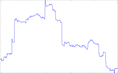
A Poisson process sample path — Figure 1: A Cauchy process sample path

Continuous-time stochastic processes with stationary independent increments are known as Lévy processes. In the previous post, it was seen that processes with independent increments are described by three terms — the covariance structure of the Brownian motion component, a drift term, and a measure describing the rate at which jumps occur. Being a special case of independent increments processes, the situation with Lévy processes is similar. However, stationarity of the increments does simplify things a bit. We start with the definition.

Definition 1 (Lévy process) A d-dimensional Lévy process X is a stochastic process taking values in ${{\mathbb R}^d}$ such that

More generally, it is possible to define the notion of a Lévy process with respect to a given filtered probability space ${(\Omega,\mathcal{F},\{\mathcal{F}_t\}_{t\ge0},{\mathbb P})}$ . In that case, we also require that X is adapted to the filtration and that ${X_t-X_s}$ is independent of ${\mathcal{F}_s}$ for all ${s < t}$ . In particular, if X is a Lévy process according to definition 1 then it is also a Lévy process with respect to its natural filtration ${\mathcal{F}_t=\sigma(X_s\colon s\le t)}$ . Note that slightly different definitions are sometimes used by different authors. It is often required that ${X_0}$ is zero and that X has cadlag sample paths. These are minor points and, as will be shown, any process satisfying the definition above will admit a cadlag modification.

The most common example of a Lévy process is Brownian motion, where ${X_t-X_s}$ is normally distributed with zero mean and variance ${t-s}$ independently of ${\mathcal{F}_s}$ . Other examples include Poisson processes, compound Poisson processes, the Cauchy process, gamma processes and the variance gamma process.

For example, the symmetric Cauchy distribution on the real numbers with scale parameter ${\gamma > 0}$ has probability density function p and characteristic function ${\phi}$ given by,

$\displaystyle \setlength\arraycolsep{2pt} \begin{array}{rl} &\displaystyle p(x)=\frac{\gamma}{\pi(\gamma^2+x^2)},\smallskip\\ &\displaystyle\phi(a)\equiv{\mathbb E}\left[e^{iaX}\right]=e^{-\gamma\vert a\vert}. \end{array}$

(1)

From the characteristic function it can be seen that if X and Y are independent Cauchy random variables with scale parameters ${\gamma_1}$ and ${\gamma_2}$ respectively then ${X+Y}$ is Cauchy with parameter ${\gamma_1+\gamma_2}$ . We can therefore consistently define a stochastic process ${X_t}$ such that ${X_t-X_s}$ has the symmetric Cauchy distribution with parameter ${t-s}$ independent of ${\{X_u\colon u\le t\}}$ , for any ${s < t}$ . This is called a Cauchy process, which is a purely discontinuous Lévy process. See Figure 1.

Lévy processes are determined by the triple ${(\Sigma,b,\nu)}$ , where ${\Sigma}$ describes the covariance structure of the Brownian motion component, b is the drift component, and ${\nu}$ describes the rate at which jumps occur. The distribution of the process is given by the Lévy-Khintchine formula, equation (3) below.

Theorem 2 (Lévy-Khintchine) Let X be a d-dimensional Lévy process. Then, there is a unique function ${\psi\colon{\mathbb R}\rightarrow{\mathbb C}}$ such that

$\displaystyle {\mathbb E}\left[e^{ia\cdot (X_t-X_0)}\right]=e^{t\psi(a)}$ (2)

for all ${a\in{\mathbb R}^d}$ and ${t\ge0}$ . Also, ${\psi(a)}$ can be written as

$\displaystyle \psi(a)=ia\cdot b-\frac{1}{2}a^{\rm T}\Sigma a+\int _{{\mathbb R}^d}\left(e^{ia\cdot x}-1-\frac{ia\cdot x}{1+\Vert x\Vert}\right)\,d\nu(x)$ (3)

where ${\Sigma}$ , b and ${\nu}$ are uniquely determined and satisfy the following,

${\Sigma\in{\mathbb R}^{d^2}}$ is a positive semidefinite matrix.

${b\in{\mathbb R}^d}$ .

${\nu}$ is a Borel measure on ${{\mathbb R}^d}$ with ${\nu(\{0\})=0}$ and,

$\displaystyle \int_{{\mathbb R}^d}\Vert x\Vert^2\wedge 1\,d\nu(x)<\infty.$ (4)

Furthermore, ${(\Sigma,b,\nu)}$ uniquely determine all finite distributions of the process ${X-X_0}$ .

Conversely, if ${(\Sigma,b,\nu)}$ is any triple satisfying the three conditions above, then there exists a Lévy process satisfying (2,3).

Proof: This result is a special case of Theorem 1 from the previous post, where it was shown that there is a continuous function ${{\mathbb R}^d\times{\mathbb R}_+\rightarrow{\mathbb C}}$ , ${(a,t)\mapsto\psi_t(a)}$ such that ${\psi_0(a)=0}$ and

$\displaystyle {\mathbb E}[e^{ia\cdot(X_t-X_0)}]=e^{\psi_t(a)}.$

Using independence and stationarity of the increments of X,

$\displaystyle \setlength\arraycolsep{2pt} \begin{array}{rl} \displaystyle e^{\psi_{s+t}(a)}&\displaystyle={\mathbb E}[e^{ia\cdot(X_{s+t}-X_t)}e^{ia\cdot(X_t-X_0}]\smallskip\\ &\displaystyle={\mathbb E}[e^{ia\cdot(X_s-X_0)}]{\mathbb E}[e^{ia\cdot(X_t-X_0)}]\smallskip\\ &\displaystyle=e^{\psi_s(a)+\psi_t(a)}. \end{array}$

So, ${\psi_{s+t}=\psi_s+\psi_t}$ and, by continuity in t, this gives ${\psi_t(a)=t\psi_1(a)}$ . Taking ${\psi(a)\equiv\psi_1(a)}$ gives (2).

Again using Theorem 1 of the previous post, there is a uniquely determined triple ${(\tilde\Sigma,\tilde b,\mu)}$ such that

$\displaystyle t\psi(a)=ia\cdot\tilde b_t-\frac12a^{\rm T}\tilde\Sigma_t a+\int_{{\mathbb R}^d\times[0,t]}\left(e^{ia\cdot x}-1-\frac{ia\cdot x}{1+\Vert x\Vert}\right)\,d\mu(x,s).$

(5)

Here, ${t\mapsto\tilde\Sigma_t}$ is a continuous function from ${{\mathbb R}_+}$ to ${{\mathbb R}^{d^2}}$ such that ${\tilde\Sigma_t-\tilde\Sigma_s}$ is positive semidefinite for all ${t > s}$ . Also, ${t\mapsto\tilde b_t}$ is a continuous function from ${{\mathbb R}_+}$ to ${{\mathbb R}^d}$ and ${\mu}$ is a Borel measure on ${{\mathbb R}^d\times{\mathbb R}_+}$ with ${\mu(\{0\}\times{\mathbb R}_+)=0}$ and

$\displaystyle \int_{{\mathbb R}^d\times[0,t]}\Vert x\Vert^2\wedge1\,d\mu(x,s) < \infty.$

Taking ${\Sigma=\tilde\Sigma_1}$ , ${b=\tilde b_1}$ and defining ${\nu}$ by ${\nu(S)=\mu(S\times[0,1])}$ it can be seen that (3) follows from (5) with ${t=1}$ , and that ${(\Sigma,b,\nu)}$ satisfy the required conditions. Conversely, if (3) is satisfied, then taking ${\tilde\Sigma_t=t\Sigma}$ , ${\tilde b_t=tb}$ and ${d\mu(x,t)=d\nu(x)\,dt}$ gives (5). Then, uniqueness of ${(\tilde\Sigma,\tilde b,\mu)}$ implies that ${(\Sigma,b,\nu)}$ are uniquely determined by (3).

Finally, if ${(\Sigma,b,\nu)}$ satisfy the required conditions, then taking ${\tilde\Sigma_t=t\Sigma}$ , ${\tilde b_t=tb}$ and ${d\mu(x,t)=d\nu(x)\,dt}$ , Theorem 1 of the previous post says that there exists an independent increments process satisfying (5). This is then the required Lévy process. ⬜

The measure ${\nu}$ above is called the Lévy measure of X, ${(\Sigma,b,\nu)}$ are referred to as the characteristics of X, and it is said to be purely discontinuous if ${\Sigma=0}$ . Note that a Lévy process with zero Lévy measure ${\nu=0}$ satisfies ${\psi(a)=ia\cdot b-\frac12a^{\rm T}\Sigma a}$ , so is a Brownian motion with covariance matrix ${\Sigma}$ and drift ${b}$ .

As an example, consider the purely discontinuous real-valued Lévy process with characteristics ${(0,0,\nu)}$ and ${d\nu(x)=\frac{dx}{\pi x^2}}$ . This satisfies (4), so determines a well-defined process. Using the Lévy-Khintchine formula we can compute its characteristic function,

$\displaystyle \setlength\arraycolsep{2pt} \begin{array}{rl} \displaystyle\psi(a)&\displaystyle=\int_{-\infty}^\infty\left(e^{ia\cdot x}-1-\frac{iax}{1+\vert x\vert}\right)\frac{dx}{\pi x^2}\smallskip\\ &\displaystyle=-\frac{4}{\pi}\int_0^\infty\frac{\sin^2(ax/2)}{x^2}\,dx\smallskip\\ &\displaystyle=-\frac{2\vert a\vert}{\pi}\int_0^\infty\frac{\sin^2 y}{y^2}\,dy=-\vert a\vert. \end{array}$

Here, the identity ${e^{iax}+e^{-iax}-2=-4\sin^2(ax/2)}$ is being used followed by the substitution ${y=\vert a\vert x/2}$ . Comparing this with the characteristic function (2) of the Cauchy distribution shows that X is the Cauchy process.

As mentioned above, Lévy processes are often taken to be cadlag by definition. However, Theorem 2 of the previous post states that all independent increments processes which are continuous in probability have a cadlag version.

Theorem 3 Every Lévy process has a cadlag modification.

We can go further than this.

Theorem 4 Every cadlag Lévy process is a semimartingale.

Proof: Theorem 2 of the previous post states that a cadlag Lévy process X decomposes as ${X_t=bt+W+Y}$ where Y is a semimartingale and W is a continuous centered Gaussian process with independent increments, hence a martingale. So, W is a semimartingale and so is X. ⬜

The characteristics of a Lévy process fully determine its finite distributions since, by equation (3), they determine the characteristic function of the increments of the process. The following theorem shows how the characteristics relate to the paths of the process and, in particular, the Lévy measure ${\nu}$ does indeed describe the jumps. This is just a specialization of Theorem 2 of the previous post to the stationary increments case.

Theorem 5 Let X be a cadlag d-dimensional Lévy process with characteristics ${(\Sigma,b,\nu)}$ . Then,

The process

$\displaystyle Y_t=X_t-X_0-\sum_{s\le t}\Delta X_s\Vert\Delta X_s\Vert / ( 1 + \Vert\Delta X_s\Vert)$ (6)

is integrable, and ${{\mathbb E}[Y_t]=tb}$ . Furthermore, ${Y_t-bt}$ is a martingale.

The quadratic variation of X has continuous part ${[X^i,X^j]^c_t=t\Sigma^{ij}}$ .

For any nonnegative measurable ${f\colon\mathbb{R}^d\rightarrow\mathbb{R}}$ ,
$\displaystyle t\nu(f)={\mathbb E}\left[\sum_{s\le t}1_{\{\Delta X_s\not=0\}}f(\Delta X_s)\right].$

In particular, for any measurable ${A\subseteq{\mathbb R}^d}$ the process

$\displaystyle X^A_t\equiv\sum_{s\le t}1_{\{\Delta X_s\in A\setminus\{0\}\}}$ (7)

is almost surely infinite for all ${t > 0}$ whenever ${\nu(A)}$ is infinite, otherwise it is a homogeneous Poisson process of rate ${\nu(A)}$ . If ${A_1,A_2,\ldots,A_n}$ are disjoint measurable subsets of ${{\mathbb R}^d}$ then ${X^{A_1},\ldots,X^{A_n}}$ are independent processes.

Furthermore, letting ${\mathcal{P}}$ be the predictable sigma-algebra and

$\displaystyle \setlength\arraycolsep{2pt} \begin{array}{rl} &\displaystyle{\mathbb R}^d\times{\mathbb R}_+\times\Omega\rightarrow{\mathbb R},\smallskip\\ &\displaystyle(x,t,\omega)\mapsto f(x,t)(\omega) \end{array}$

be ${\mathcal{B}({\mathbb R}^d)\otimes\mathcal{P}}$ -measurable such that ${f(0,t)=0}$ and ${\int_0^t\int_{{\mathbb R}^d}\vert f(x,s)\vert\,d\nu(x)ds}$ is integrable (resp. locally integrable) then,

$\displaystyle M^f_t\equiv\sum_{s\le t}f(\Delta X_s,s)-\int_0^t\int_{{\mathbb R}^d}f(x,s)\,d\nu(x)ds$ (8)

is a martingale (resp. local martingale).

Proof: The first statement follows directly from the first statement of Theorem 2 of the previous post.

Now apply the decomposition ${X=bt+W+Y}$ from the second statement of Theorem 2 of the previous post, where W has quadratic variation ${[W^i,W^j]_t=\Sigma^{ij}t}$ and Y satisfies ${[Y^i,Y^j]^{\rm c}=0}$ . This gives ${[X^i,X^j]^{\rm c}_t=[W^i,W^j]_t=\Sigma^{ij}t}$ as required.

For the third statement above, define the measure ${d\mu(x,t)=d\nu(x)\,dt}$ on ${{\mathbb R}^d\times{\mathbb R}_+}$ . By the third statement of Theorem 2 of the previous post,

$\displaystyle {\mathbb E}\left[\sum_{s\le t}1_{\{\Delta X_s\not=0\}}f(\Delta X_s)\right]=\int f(x,s)1_{\{s\le t\}}\,d\mu(x,s)=t\nu(f).$

Also, as stated in Theorem 2 of the previous post, for a measurable ${A\subseteq{\mathbb R}^d\times{\mathbb R}_+}$ , the random variable

$\displaystyle \eta(A)\equiv\sum_{t > 0}1_{\{\Delta X_t\not=0,(\Delta X_t,t)\in A\}}$

is almost surely infinite whenever ${\mu(A)=\infty}$ and Poisson distributed of rate ${\mu(A)}$ otherwise. Furthermore, ${\eta(A_1),\ldots,\eta(A_n)}$ are independent whenever ${A_1,\ldots,A_n}$ are disjoint measurable subsets of ${{\mathbb R}^d\times{\mathbb R}_+}$ . We can apply this to the process ${X^A_t=\eta(A\times[0,t])}$ defined by (7).

If ${A\subseteq{\mathbb R}^d}$ satisfies ${\nu(A)=\infty}$ then ${\mu(A\times[0,t])=t\nu(A)}$ is infinite for all ${t > 0}$ , so ${X^A_t}$ is almost surely infinite. On the other hand, if ${\nu(A)}$ is finite, consider a sequence of times ${0\le t_0 < t_1 <\cdots < t_n}$ . The increments of ${X^A}$ are ${X^A_{t_k}-X^A_{t_{k-1}}=\eta(A\times(t_{k-1},t_k])}$ which are independent and Poisson distributed with rates ${\mu(A\times(t_{k-1},t_k])=\nu(A)(t_k-t_{k-1})}$ . So, ${X^A}$ is a homogeneous Poisson process of rate ${\nu(A)}$ .

If ${A_1,\ldots,A_n}$ are disjoint measurable subsets of ${{\mathbb R}^d}$ , then ${X^{A_k}}$ are Poisson processes (whenever ${\nu(A_k) < \infty}$ ) and, by construction, no two can ever jump simultaneously. So, they are independent.

Finally, that (8) is a (local) martingale is given by the final statement of Theorem 2 of the previous post. ⬜

The following characterization of the purely discontinuous Lévy processes is an immediate consequence of the second statement of Theorem 5.

Corollary 6 A cadlag Lévy process X is purely discontinuous if and only if its quadratic variation has zero continuous part, ${[X^i,X^j]^{\rm c}=0}$ .

Any Lévy process decomposes uniquely into its continuous and purely discontinuous parts.

Lemma 7 A cadlag Lévy process X decomposes uniquely as ${X=W+Y}$ where W is a continuous centered Gaussian process with independent increments, ${W_0=0}$ , and Y is a purely discontinuous Lévy process.

Furthermore, W and Y are independent and if X has characteristics ${(\Sigma,b,\nu)}$ then W and Y have characteristics ${(\Sigma,0,0)}$ and ${(0,b,\nu)}$ respectively.

Proof: Theorem 2 of the previous post says that X decomposes uniquely as ${X_t=bt+W_t+\tilde Y_t}$ where W is a continuous centered Gaussian process with independent increments, ${W_0=0}$ , and Y is a semimartingale with independent increments whose quadratic variation has zero continuous part ${[Y^i,Y^j]^{\rm c}=0}$ . Furthermore, W and ${\tilde Y}$ are independent Lévy processes with characteristics ${(\Sigma,0,0)}$ and ${(0,0,\nu)}$ respectively.

So, taking ${Y_t=bt+\tilde Y}$ gives the required decomposition, satisfying the required properties. Conversely, supposing that ${X=W^\prime+Y^\prime}$ is any other such decomposition, uniqueness of the decomposition ${X_t=bt+W_t+\tilde Y_t=bt + W^\prime_t+(Y^\prime_t-bt)}$ gives ${W=W^\prime}$ and ${Y^\prime_t=\tilde Y_t+bt=Y_t}$ . ⬜

Recall that for any independent increments process X which is continuous in probability, the space-time process ${(X_t,t)}$ is Feller. For Lévy processes, where the increments of X are stationary, we can use a very similar proof to show that X itself is a Feller process.

Lemma 8 Let X be a d-dimensional Lévy process. For each ${t\ge0}$ define the transition probability ${P_t}$ on ${{\mathbb R}^d}$ by

$\displaystyle P_tf(x)={\mathbb E}\left[f(X_t-X_0+x)\right]$

for nonnegative measurable ${f\colon{\mathbb R}^d\rightarrow{\mathbb R}}$ .

Then, X is a Markov process with Feller transition function ${\{P_t\}_{t\ge0}}$ .

Proof: To show that ${P_t}$ defines a Markov transition function, the Chapman-Kolmogorov equations ${P_sP_t=P_{s+t}}$ need to be verified. The stationary independent increments property gives

$\displaystyle P_tf(x)={\mathbb E}[f(X_{s+t}-X_s+x)]={\mathbb E}[f(X_{s+t}-X_s+x)\mid\mathcal{F}_s]$

(9)

for times ${s,t\ge 0}$ . As the expectation is conditioned on ${\mathcal{F}_s}$ , we can replace x by any ${\mathcal{F}_s}$ -measurable random variable. In particular,

$\displaystyle P_tf(X_s-X_0+x)={\mathbb E}[f(X_{s+t}-X_0+x)\mid\mathcal{F}_s].$

This gives

$\displaystyle P_sP_tf(x)={\mathbb E}[P_tf(X_s-X_0+x)]={\mathbb E}[f(X_{s+t}-X_0+x)]=P_{s+t}f(x)$

as required. So, ${P_t}$ defines a Markov transition function. Replacing x by ${X_s}$ in (9) gives

$\displaystyle P_tf(X_s)={\mathbb E}[f(X_{s+t}\mid\mathcal{F}_s],$

so X is Markov with transition function ${P_t}$ .

It only remains needs to be shown that ${P_t}$ is Feller. That is, for ${f\in C_0({\mathbb R}^d)}$ , ${P_tf\in C_0({\mathbb R}^d)}$ and ${P_tf(x)\rightarrow f(x)}$ as ${t\rightarrow0}$ . Letting ${x_n\in{\mathbb R}^d}$ tend to a limit ${x}$ , bounded convergence gives

$\displaystyle P_tf(x_n)={\mathbb E}[f(X_t-X_0+x_n)]\rightarrow{\mathbb E}[f(X_t-X_0+x)]=P_tf(x)$

as ${n\rightarrow\infty}$ . So, ${P_tf}$ is continuous. Similarly, if ${\Vert x_n\Vert\rightarrow\infty}$ then ${f(X_t-X_0+x_n)}$ tends to zero, giving ${P_tf(x_n)\rightarrow0}$ . So, ${P_tf}$ is in ${C_0({\mathbb R}^d)}$ .

Finally, if ${t_n\ge0}$ is a sequence of times tending to zero then ${X_{t_n}\rightarrow X_0}$ in probability, giving

$\displaystyle P_{t_n}f(x)={\mathbb E}[f(X_{t_n}-X_0+x)]\rightarrow f(x)$

as required. ⬜

Finally, we can calculate the infinitesimal generator of a Lévy process in terms of its characteristics.

Theorem 9 Let X be a d-dimensional Lévy process with characteristics ${(\Sigma,b,\nu)}$ and define the operator A on the bounded and twice continuously differentiable functions ${C^2_b({\mathbb R}^d)}$ from ${{\mathbb R}^d}$ to ${{\mathbb R}}$ as

$\displaystyle Af(x) = b^if_i(x) - \frac12\Sigma^{ij}f_{ij}(x)+\int\left(f(x+y)-f(x)-\frac{y^if_i(x)}{1+\Vert y\Vert}\right)\,d\nu(y).$ (10)

Then,

$\displaystyle M_t=f(X_t)-\int_0^t Af(X_s)\,ds$

is a local martingale for all ${f\in C^2_b({\mathbb R}^d)}$ .

In equation (10) the summation convention is being used, so that if i or j appears twice in a single term then it is summed over the range ${1,2,\ldots,d}$ .

Proof: Apply the generalized Ito formula to ${f(X)}$ ,

$\displaystyle \setlength\arraycolsep{2pt} \begin{array}{rl} \displaystyle dM_t=&\displaystyle f_i(X_{t-})(dX^i_t -b^i\,dt)+\frac12f_{ij}(X_{t-})(d[X^i,X^j]^{\rm c}_t-\Sigma^{ij}\,dt)\smallskip\\ &\displaystyle+\left(\Delta f(X_t)-f_i(X_{t-})\Delta X^i_t\right)\smallskip\\ &\displaystyle\qquad-\int\left(f(X_t+y)-f(X_{t-})-\frac{y^if_i(X_t)}{1+\Vert y\Vert}\right)\,d\nu(y)dt. \end{array}$

(11)

Now define the ${\mathcal{B}({\mathbb R}^d)\otimes\mathcal{P}}$ -measurable function g by

$\displaystyle g(y,t)=f(X_{t-}+y)-f(X_{t-})-y^if_i(X_{t-})/(1+\Vert y\Vert)$

and let ${M^g}$ be the local martingale defined as in (8). Also, define Y by (6). Then, using the identity ${[X^i,X^j]^{\rm c}_t=\Sigma^{ij}t}$ , equation (11) can be rewritten as

$\displaystyle dM_t = f_i(X_{t-})\,d(Y^i_t-b^it)-dM^g_t.$

As ${Y_t-bt}$ is a martingale, this shows that M is a local martingale. ⬜

In particular, if f is in the space ${C^2_0({\mathbb R}^d)}$ of twice continuously differentiable functions vanishing at infinity and ${Af\in C_0({\mathbb R}^d)}$ then Theorem 9 shows that f is in the domain of the generator of the Feller process X, and A is the infinitesimal generator. So,

$\displaystyle Af=\lim_{t\rightarrow0}\frac1t\left(P_tf-f\right),$

where convergence is uniform on ${{\mathbb R}^d}$ . For any Lévy process for which the distribution of ${X_t}$ is known, this allows us to compute ${Af}$ and, then, read off the Lévy characteristics. In particular, if ${f\colon{\mathbb R}^d\rightarrow{\mathbb R}}$ is twice continuously differentiable with compact support contained in ${{\mathbb R}^d\setminus\{0\}}$ then,